Chapter 4 Orthogonality
4.1 Dot Product, Norm, and Euclidean Distance
Definition 4.1 (transpose) Let \(A \in \mathrm{M}_{m,n}(\mathbf{R})\), the transpose of \(A\) is the matrix \(^tA \in \mathrm{M}_{n,m}(\mathbf{R})\) given by
\[ (^tA)_{i,j} = A_{j,i} \]
for all \(1 \leq i \leq n\) and \(1 \leq j \leq m\).
Remark. The transpose corresponds to exchanging the rows with the columns.
Example 4.1 The transpose of a column vector \(X = \begin{bmatrix} X_1 \\ \dots \\ X_n \end{bmatrix}\) is the row vector \(^tX = \begin{bmatrix} X_1, \dots, X_n \end{bmatrix}\).
Example 4.2 The transpose of the matrix
\[ A = \begin{bmatrix} 1 & 0 & 2 \\ 3 & 2 & 1 \end{bmatrix} \] is the matrix
\[ ^tA = \begin{bmatrix} 1 & 3 \\ 0 & 2 \\ 2 & 1 \end{bmatrix}. \]
Proposition 4.1 If \(A \in \mathrm{M}_{n,m}(\mathbf{K})\) and \(B \in \mathrm{M}_{m,l}(\mathbf{K})\), then \(^t(AB) = (^tB)(^tA)\).
Proof. The coefficient at index \((i,j)\) of \(AB\) is \(\sum_{k=1}^m A_{i,k}B_{k,j}\), so the coefficient at index \((i,j)\) of \(^t(AB)\) is \(\sum_{k=1}^m A_{j,k}B_{k,i}\).
The coefficient of \((^tB)(^tA)\) at index \((i,j)\) is
\[\begin{align*} \sum_{k=1}^m (^tB)_{i,k} (^tA)_{k,j} &= \sum_{k=1}^m B_{k,i}A_{j,k} \\ &= \sum_{k=1}^m A_{j,k}B_{k,i}. \end{align*}\]
The matrices \(^t(AB)\) and \((^tB)(^tA)\) have the same coefficients, so they are equal.
Definition 4.2 (dot product) Let \(u, v\) be two vectors in \(\mathbf{R}^n\). The dot product of \(u\) and \(v\) is the real number
\[ \langle u, v \rangle = \sum_{i=1}^n u_i v_i \]
where \((u_i)\) and \((v_i)\) are the coordinates of \(u\) and \(v\) in the canonical basis.
Remark. If \(X\) and \(Y\) are column vectors in \(\mathbf{R}^n\), then \(\langle X, Y \rangle\) is identified with the \(1 \times 1\) matrix \(^tXY\).
Proposition 4.2 For all \(u, v, w \in \mathbf{R}^n\) and \(\lambda \in \mathbf{R}\), the following properties hold:
- \(\langle u, v \rangle = \langle v, u \rangle\),
- \(\langle u + v, w \rangle = \langle u, w \rangle + \langle v, w \rangle\),
- \(\langle \lambda u, v \rangle = \lambda \langle u, v \rangle\),
- \(\langle u, u \rangle \geq 0\),
- \(\langle u, u \rangle = 0 \iff u = 0\).
Proof. We prove the properties one after the other:
- \(\langle u, v \rangle = \sum_{i=1}^n u_i v_i = \sum_{i=1}^n v_i u_i = \langle v, u \rangle\),
- \(\langle u + v, w \rangle = \sum_{i=1}^n (u_i + v_i) w_i = \sum_{i=1}^n u_i w_i + \sum_{i=1}^n v_i w_i = \langle u, w \rangle + \langle v, w \rangle\),
- \(\langle \lambda u, v \rangle = \sum_{i=1}^n \lambda u_i v_i = \lambda \sum_{i=1}^n u_i v_i = \lambda \langle u, v \rangle\),
- \(\langle u, u \rangle = \sum_{i=1}^n u_i^2 \geq 0\),
- \(\langle u, u \rangle = \sum_{i=1}^n u_i^2 = 0 \iff \forall i,\ u_i = 0 \iff u = 0\).
Definition 4.3 (euclidean norm) Let \(u \in \mathbf{R}^n\), the Euclidean norm (or simply norm) of \(u\) is the positive real number
\[ ||u|| = \sqrt{\langle u, u \rangle} = \sqrt{\sum_{i=1}^n u_i^2}. \]
Remark. The last property of Proposition 4.2 shows that \(||u|| = 0 \iff u = 0\).
Definition 4.4 (euclidean distance) Let \(u, v \in \mathbf{R}^n\), the Euclidean distance (or simply distance) between \(u\) and \(v\) is the positive real number
\[ d(u, v) = ||u - v|| = \sqrt{\sum_{i=1}^n (u_i - v_i)^2}. \]
Remark. The norm \(||u||\) of a vector \(u\) is thus the distance from \(u\) to 0.
4.2 Orthogonality
Definition 4.5 Let \(u, v\) be two vectors in \(\mathbf{R}^n\). They are orthogonal if \(\langle u, v \rangle = 0\).
We then write \(u \bot v\).
Example 4.3 If \(u = \begin{bmatrix} 1 \\ 1 \end{bmatrix}\) and \(v = \begin{bmatrix} 1 \\ -1 \end{bmatrix}\), then \(u\) and \(v\) are orthogonal because \(\langle u, v \rangle = 1 - 1 = 0\).
Example 4.4 The vectors \(e_1, \dots, e_n\) of the canonical basis are orthogonal because \(\langle e_i, e_j \rangle = 1\) if \(i = j\) and \(\langle e_i, e_j \rangle = 0\) if \(i \neq j\).
Definition 4.6 Let \(E\) be a subset of \(\mathbf{R}^n\). The orthogonal of \(E\) is the set
\[\{y \in \mathbf{R}^n \mid \forall x \in E, \langle x, y \rangle = 0\}.\] It is denoted \(E^\bot\). If \(u \in E^\bot\), we also write \(u \bot E\).
Lemma 4.1 The set \(E^\bot\) is a vector subspace of \(\mathbf{R}^n\).
Proof. Let \(y_1, y_2 \in E^\bot\). For all \(x \in E\), \(\langle y_1 + y_2, x \rangle = \langle y_1, x \rangle + \langle y_2, x \rangle = 0\), so \(y_1 + y_2 \in E^\bot\). If \(y \in E^\bot\) and \(\lambda \in \mathbf{R}\), \(\langle \lambda y, x \rangle = \lambda \langle y, x \rangle = 0\), so \(\lambda y \in E^\bot\).
Definition 4.7 A set \(F = \{u_1, \dots, u_k\}\) is orthogonal if for all \(i, j\), \(u_i \bot u_j\).
Lemma 4.2 Let \(F\) be an orthogonal set of non-zero vectors. Then \(F\) is linearly independent.
Proof. Let \(u_1, \dots, u_k \in F\) and \(\lambda_1, \dots, \lambda_k \in \mathbf{R}\) such that \[\lambda_1 u_1 + \dots + \lambda_k u_k = 0.\] We want to show that \(\lambda_1 = \dots = \lambda_k = 0\). Let \(v = \lambda_1 u_1 + \dots + \lambda_k u_k\) and compute \(\langle v, u_i \rangle\). Since \(v = 0\), \(\langle v, u \rangle = 0\), and by linearity, \(\langle v, u_i \rangle = \sum_{j = 1}^k \lambda_j \langle u_j, u_i \rangle = \lambda_i \langle u_i, u_i \rangle\) for a fixed \(i\). Since \(u_i \neq 0\), \(\langle u_i, u_i \rangle \neq 0\), so \(\lambda_i = 0\). This shows that the set is linearly independent.
Definition 4.8 A basis \(\mathcal{B} = (u_1, \dots, u_n)\) of \(\mathbf{R}^n\) is orthonormal if for all \(i \neq j\), \(u_i \bot u_j\), and \(||u_i|| = 1\) for all \(i \in \{1, \dots, n\}\).
Remark. By Lemma 4.2, an orthogonal set with \(n\) vectors of norm 1 is automatically an orthonormal basis.
Example 4.5 The canonical basis is an orthonormal basis.
Example 4.6 The set \(u_1 = \frac{1}{\sqrt{2}} \begin{bmatrix} 1 \\ 1 \end{bmatrix}\) and \(u_2 = \frac{1}{\sqrt{2}} \begin{bmatrix} -1 \\ 1 \end{bmatrix}\) is an orthonormal basis because \(||u_1|| = ||u_2|| = 1\) and \(u_1 \bot u_2\).
4.3 Projections and Closest Point
Definition 4.9 Let \(u\) be a vector in \(\mathbf{R}^n\) and let \(D\) be the line generated by \(u\). The projection of a vector \(v \in \mathbf{R}^n\) onto \(D\) is the vector \(\frac{\langle u,v\rangle}{\langle u,u\rangle}u\). It is denoted as \(P_D(v)\).
Definition 4.10 Let \(E\) be a vector subspace of \(\mathbf{R}^n\), and \(u_1, \dots, u_k\) be an orthonormal basis of \(E\). The projection of a vector \(v\) onto \(E\) is the vector \(P_E(v)=\sum_{i=1}^k \langle v,u_i \rangle u_i \in E\).
Remark. This is the sum of the projections onto the lines generated by \(u_i\).
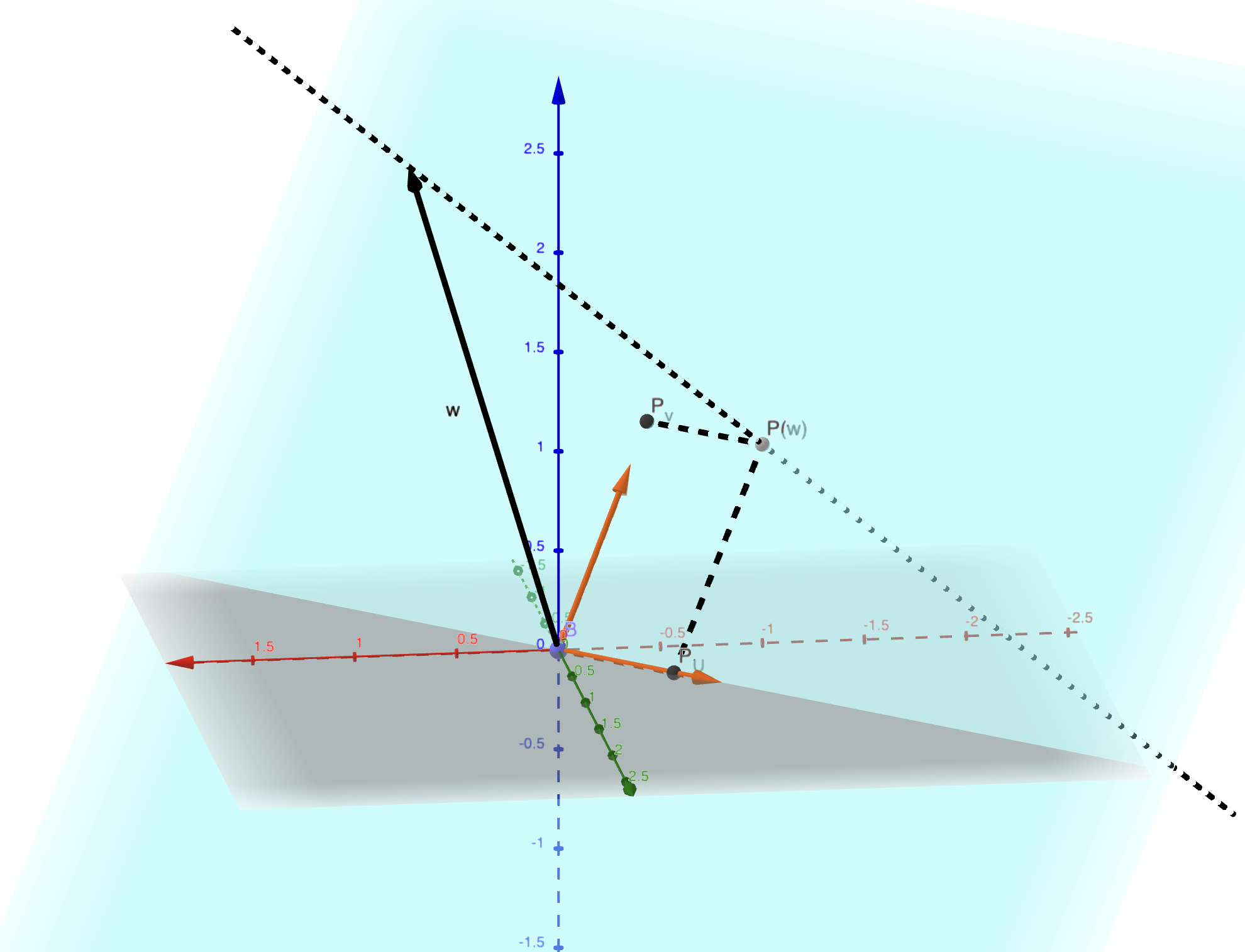
Figure 4.1: The projection of vector w onto a plane.
Lemma 4.3 Let \(E\) be a vector subspace of \(\mathbf{R}^n\). The map \(u \mapsto P_E(u)\) is a linear application.
Proof. Let \(v_1,v_2 \in \mathbf{R}^n\). Then
\[ P_E(v_1+v_2) = \sum_{i=1}^k \langle v_1+v_2, u_i \rangle u_i = P_E(v_1) + P_E(v_2) \]
For \(\lambda \in \mathbf{R}\) and \(v \in \mathbf{R}^n\),
\[ P_E(\lambda v) = \lambda P_E(v) \]
Thus, the orthogonal projection onto \(E\) is a linear application.
Lemma 4.4 Let \(E\) be a vector subspace of \(\mathbf{R}^n\) and \(v \in \mathbf{R}^n\). Then \(v - P_E(v) \in E^\bot\) and
\[||v||^2 = ||P_E(v)||^2 + ||v - P_E(v)||^2.\]
Proof. Let \(v_\bot = v - P_E(v)\). Then \(v = P_E(v) + v_\bot\).
For \(i \in \{1,\dots,k\}\),
\[ \langle u_i, v_\bot \rangle = \langle v, u_i \rangle - \langle P_E(v), u_i \rangle = 0 \]
Thus, \(v_\bot = v - P_E(v) \in E^\bot\).
Now,
\[ ||v||^2 = ||P_E(v)||^2 + ||v - P_E(v)||^2. \]
Lemma 4.5 (Cauchy-Schwarz Inequality) For \(u,v \in \mathbf{R}^n\), we have
\[|\langle u,v\rangle| \leq ||u||||v||.\]
Proof. By construction, we have \(\langle u,v \rangle = \langle P_D(u), v \rangle\) where \(D\) is the line generated by \(v\). Since \(||P_D(u)|| \leq ||u||\), the result follows.
Proposition 4.3 (Triangle Inequality) For \(u,v \in \mathbf{R}^n\), we have
\[||u+v|| \leq ||u|| + ||v||.\]
Remark. Let \(a, b, c\) be three points in \(\mathbf{R}^n\). Using \(u = a - b\) and \(v = b - c\), we obtain
\[d(a,c) \leq d(a,b) + d(b,c).\]
Proof. We compute \(||u + v||^2\):
\[ ||u + v||^2 = ||u||^2 + 2\langle u,v \rangle + ||v||^2 \leq (||u|| + ||v||)^2 \]
Thus, \(||u + v|| \leq ||u|| + ||v||.\)
Proposition 4.4 Let \(E\) be a vector subspace of \(\mathbf{R}^n\) and \(u \in \mathbf{R}^n\). For all \(v \in E\),
\[||u - v|| \geq ||u - P_E(u)||.\]
Remark. This means that \(P_E(u)\) is the closest point in \(E\) to \(u\). In particular, this point \(P_E(u)\) does not depend on the orthonormal basis chosen to define it.
Definition 4.11 (Gram-Schmidt Orthogonalization) Let \(u_1, \dots, u_k\) be a basis of a subspace \(F\) of \(\mathbf{R}^n\). The vectors are defined by recurrence as follows:
\[\begin{align*} v_1 &= u_1 \\ v_2 &= u_2 - \frac{\langle u_2, v_1 \rangle}{\langle v_1, v_1 \rangle} v_1 \\ v_3 &= u_3 - \frac{\langle u_3, v_1 \rangle}{\langle v_1, v_1 \rangle} v_1 - \frac{\langle u_3, v_2 \rangle}{\langle v_2, v_2 \rangle} v_2 \\ \vdots &= \vdots \\ v_k &= u_k - \frac{\langle u_k, v_1 \rangle}{\langle v_1, v_1 \rangle} v_1 - \dots - \frac{\langle u_k, v_{k-1} \rangle}{\langle v_{k-1}, v_{k-1} \rangle} v_{k-1} \end{align*}\]
Finally, set \(e_i = \frac{v_i}{\|v_i\|}\).
Theorem 4.1 The set \((e_1, \dots, e_k)\) is an orthonormal basis of \(F\).
Proof. We prove by induction on \(i = 1, \dots, k\) that \((e_1, \dots, e_i)\) is an orthonormal basis of \(\mathrm{Vect}(e_1, \dots, e_i)\).
Base case \(k=1\): the vector \(e_1\) is non-zero and has norm 1.
Inductive step: Assume the result for \(k-1\). It remains to show that \(e_k\) is orthogonal to \(e_i\) for \(i < k\) since \(\|e_k\| = 1\), which is equivalent to \(v_k\) being orthogonal to \(v_i\) for \(i < k\). We calculate \(\langle v_k, v_i \rangle = \langle u_k, v_i \rangle - \frac{\langle u_k, v_i \rangle}{\langle v_i, v_i \rangle} \langle v_i, v_i \rangle = 0\).
Example 4.7 Let \(F\) be the plane defined by \(x + y + z = 0\) and \(v = (1, 2, 3)\). We want to calculate the orthogonal projection of \(v\) onto \(F\). We start by calculating an orthonormal basis for this. The vectors \(u_1 = (1, -1, 0)\) and \(u_2 = (0, 1, -1)\) form a basis of \(F\).
Applying the Gram-Schmidt orthonormalization process, we get \(v_1 = u_1\) and \(e_1 = \left(\frac{1}{\sqrt{2}}, \frac{-1}{\sqrt{2}}, 0\right)\), then \(v_2 = u_2 + \frac{1}{2}u_1 = \left(\frac{1}{2}, \frac{1}{2}, -1\right)\) and finally \(e_2 = \sqrt{\frac{2}{3}} \left(\frac{1}{2}, \frac{1}{2}, -1\right) = \left(\frac{1}{\sqrt{6}}, \frac{1}{\sqrt{6}}, -\frac{2}{\sqrt{6}}\right)\).
Since \(\langle v, e_1 \rangle = -\frac{1}{\sqrt{2}}\) and \(\langle v, e_2 \rangle = -\frac{3}{\sqrt{6}}\), we get
\[\begin{align*} P_F(v) &= \frac{-1}{\sqrt{2}} e_1 - \frac{3}{\sqrt{6}} e_2 \\ &= (-1, 0, 1). \end{align*}\]
4.4 Orthogonal Matrices
Definition 4.12 (Orthogonal Matrix) Let \(A \in \mathrm{M}_n(\mathbf{R})\). The matrix \(A\) is orthogonal if \(^tAA = I_n\).
Lemma 4.6 Let \(A \in \mathrm{M}_n(\mathbf{R})\). Denote \(A_1, \dots, A_n\) as the column vectors of the matrix \(A\). Let \(P\) be the matrix \(^tAA\). The coefficient at index \((i,j)\) of \(P\) is \(\langle A_i, A_j \rangle\).
Proof. Let \(B = ^tA\). By the definition of matrix multiplication, the coefficient \(P_{i,j}\) of \(P\) is \(\sum_{k=1}^n B_{i,k} A_{k,j}\). Since \(B_{i,k} = A_{k,i}\), \(P_{i,j} = \sum_{k=1}^n A_{k,i} A_{k,j} = \langle A_i, A_j \rangle\).
Proposition 4.5 A matrix \(A\) is orthogonal if and only if \(A\) is invertible with inverse \(^tA\) if and only if the columns of \(A\) form an orthonormal basis.
Proof. The matrix equation \(^tAA = I_n\) means exactly that \(^tA\) is the inverse of \(A\).
By Lemma 4.6, let \(P = ^tAA\). Thus, the coefficient \(P_{i,j}\) is \(\langle A_i, A_j \rangle\). Thus, \[P = I_n \iff \left\{\begin{matrix}\langle A_i, A_j \rangle = 0, \text{ for } i \neq j\\ \langle A_i, A_j \rangle = 1, \text{ for } i = j \end{matrix}\right. .\] This means exactly that the set of columns of matrix \(A\) is an orthonormal basis.
Remark. An orthogonal matrix corresponds exactly to a change of basis matrix from the standard basis to an orthonormal basis.
Example 4.8 Here are some examples.
- The matrix \(\frac{1}{\sqrt{2}} \begin{bmatrix} 1 & -1 \\ 1 & 1 \end{bmatrix}\) is an orthogonal matrix in dimension 2.
- The matrix \(\begin{bmatrix} 0 & 1 & 0 \\ 0 & 0 & 1 \\ 1 & 0 & 0 \end{bmatrix}\) is orthogonal in dimension 3.
- The matrix \(\frac{1}{9} \begin{bmatrix} -8 & 4 & 1 \\ 4 & 7 & 4 \\ 1 & 4 & -8 \end{bmatrix}\) is orthogonal in dimension 3.
Proposition 4.6 Let \(A\) be an orthogonal matrix in \(\mathbf{R}^n\). For all vectors \(X, Y \in \mathbf{R}^n\), we have
\[ \langle AX, AY \rangle = \langle X, Y \rangle. \]
Proof. We have \(\langle AX, AY \rangle = ^t(AX) AY = ^tX ^tA A Y = ^tXY = \langle X, Y \rangle\).
Corollary 4.1 Orthogonal changes of basis preserve orthogonality, norms, and distances: For all \(X, Y \in \mathbf{R}^n\) and orthogonal matrix \(A\):
- \(X \bot Y \iff AX \bot AY\),
- \(\|AX\| = \|X\|\), and
- \(d(AX, AY) = d(X, Y)\).
Proof. We have
- \(X \bot Y \iff \langle X, Y \rangle = 0 \iff \langle AX, AY \rangle = 0 \iff AX \bot AY\),
- \(\|AX\|^2 = \langle AX, AX \rangle = \langle X, X \rangle = \|X\|^2\), and
- \(d(AX, AY) = \|AX -AY\| = \|A(X - Y)\| = \|X - Y\| = d(X, Y)\).
4.5 Exercises
Exercise 4.1 (Pythagorean Theorem) Let \(u, v \in \mathbf{R}^n\).
- Show that \(\|u + v\|^2 = \|u\|^2 + 2 \langle u, v \rangle + \|v\|^2\).
- Deduce that \(u \bot v \iff \|u + v\|^2 = \|u\|^2 + \|v\|^2\).
- What is the connection with the Pythagorean theorem?
Exercise 4.2 Consider the vectors \(u_1 = (1, 0, 1)\), \(u_2 = (1, 1, 1)\), and \(u_3 = (-1, 1, 0)\). Apply the Gram-Schmidt process to the set \((u_1, u_2, u_3)\).
Exercise 4.3 In \(\mathbf{R}^3\), consider the vectors \(v_1 = (1, 1, 0)\) and \(v_2 = (1, 1, 1)\). Let \(F = \mathrm{Span}(v_1, v_2)\).
- Find an orthonormal basis for \(F\) using the Gram-Schmidt orthonormalization process.
- Calculate the image of the standard basis vectors under the orthogonal projection onto \(F\), denoted \(P_F\).
- Deduce the matrix of \(P_F\) in the standard basis.
- Provide a system of equations defining \(F^\bot\).
- Provide an orthonormal basis for \(F^\bot\).
- What is the distance from the vector \((1, -1, 1)\) to \(F\)?
Exercise 4.4 Verify that the matrix \(A = \frac{-1}{3} \begin{bmatrix} -2 & 1 & 2 \\ 2 & 2 & 1 \\ 1 & -2 & 2 \end{bmatrix}\) is an orthogonal matrix.
Exercise 4.5 In \(\mathbf{R}^3\), consider the point \(C = (1, 2, 1)\).
- Provide an equation for the sphere \(S\) centered at \(C\) with radius 2, i.e., the set of points at distance 2 from \(C\).
- Provide an equation for \(C^\bot\). What is the dimension of this subspace? Give an orthonormal basis for it.
- Represent \(S\) and \(C^\bot\) using Geogebra 3D.
- Justify that \(C^\bot \cap S = \emptyset\).
Exercise 4.6 Let \(\mathcal{B} = (u_1, \dots, u_n)\) be a basis of \(\mathbf{R}^n\) and \(\mathcal{B}' = (e_1, \dots, e_n)\) the orthonormal basis obtained by the Gram-Schmidt process. Let \(R\) be the change-of-basis matrix from \(\mathcal{B}'\) to \(\mathcal{B}\).
- Provide the entries of \(R\).
- Observe that \(R\) is an upper triangular matrix.
- Let \(Q\) be the change-of-basis matrix from the standard basis \(\mathcal{B}_0\) to \(\mathcal{B}'\). Justify that \(Q\) is an orthogonal matrix.
- Let \(A\) be an invertible matrix in \(\mathrm{M}_n(\mathbf{R})\). Denote \(u_1, \dots, u_n\) as its column vectors. Interpreting \(A\) as the change-of-basis matrix from \(\mathcal{B}_0\) to \(\mathcal{B}\), justify that \(A = QR\).
- Justify that the solution to a linear system \(AX = B\), where \(X \in \mathbf{R}^n\) is the unknown and \(B \in \mathbf{R}^n\) is given, is solved by \(X = R^{-1} (^tQ) B\), and that this is computed quite easily.