CBLasso implementation (vs BLasso)

Contents

This script compares the CBlasso and the Blasso recovery in the case of a 3-spikes measure. The architecture is the following
1) We solve the SDP dual formulation of Blasso and CBlasso. For this step, 'cvx' solver is used.
2) We proceed to roots-finding for the previous computed dual polynomial. In this step, we identify a set of locations in which the support of the measure to reconstruct is included.
3) CBlasso : we alternate between Lasso steps and noise estimation
3bis) Blasso : we proceed to a Lasso step

Some parts of this code heavily rely on the following works :
(i) http://www.cims.nyu.edu/~cfgranda/scripts/superres_sdp.m
(ii) http://nbviewer.jupyter.org/github/gpeyre/numerical-tours/blob/master/matlab/sparsity_8_sparsespikes_measures.ipynb

Developers : Claire Boyer, Yohann de Castro, Joseph Salmon (june 2016)
clear all
close all

addpath(genpath('~/Documents/MATLAB/cvx')) ;
addpath('math_tools/') ;

rng(1);

% Display features
ms = 20;
lw = 1;
P = 2048*8;
u = (0:P-1)'/P;
Data generation
fc = 80;
delta = 3/fc; % parameter for safe separation condition
N = 2*fc+1;

Fourier = @(fc,x)exp(-2i*pi*(-fc:fc)'*x(:)');

Phi  = @(fc,x,a)Fourier(fc,x)*a;
PhiS = @(fc,u,p)real( Fourier(fc,u)'* p );

% True signal
x0 = [.5-delta .5 .5+2*delta]'; % spike positions
a0 = [1 1 -1]'; % spike magnitudes
n = length(x0);
Phix0 = Phi(fc,x0,a0) ;

% Noisy observations
sigma = 1  ;
w = randn(N,1) + 1i * randn(N,1);
w = sigma * w;
y = Phix0 + w;

% Plot data
f0 = PhiS(fc,u,Phix0);
f = PhiS(fc,u,y);
figure(1);
hold on;
set(gca,'FontSize',16)
plot(u, [f0 f]);
stem(x0, 10*sign(a0), 'k.--', 'MarkerSize', ms, 'LineWidth', 1);
axis tight; box on;
h=legend('${\mathcal{F}_n}^* \left( {\mathcal{F}_n} (\mu^0) \right)$', '${\mathcal{F}_n}^* y$');
set(h,'Interpreter','latex')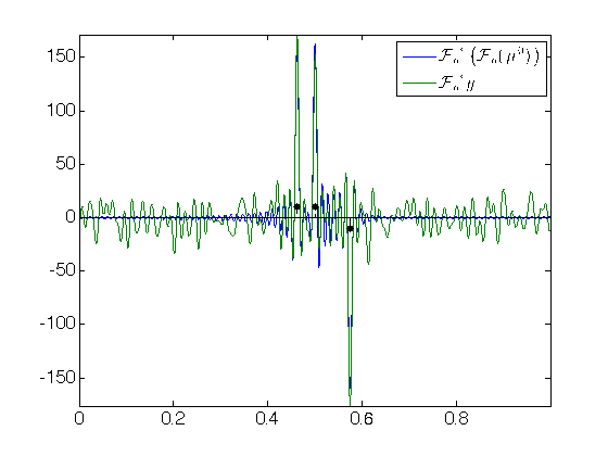
 
Blasso - constructing the dual polynomial
% Parameters for SDP resolution
q = ones(N,1);
alpha = 2 ;

% SDP Blasso
lambda_max_blasso = norm(PhiS(fc,u,y),inf) / N ;
lambda_blasso = N * lambda_max_blasso/alpha;
tic
cvx_solver sdpt3 % SeDuMi %
        cvx_begin sdp quiet
        cvx_precision high;
        variable X(N+1,N+1) hermitian;
        variable c(N) complex;
        X >= 0;
        X(N+1,N+1) == 1;
        X(1:N,N+1) == c .* conj(q);
        trace(X) == 2;
        for j = 1:N-1,
            sum(diag(X,j)) == X(N+1-j,N+1);
        end
        if lambda_blasso==0
            maximize(real( c' * y ))
        else
            minimize( norm(y/lambda_blasso-c, 'fro') )
        end
        cvx_end
Blasso_coeff = X(1:N,N+1);
toc

% Plot the Blasso polynomial

etaLambda_Blasso = PhiS(fc,u,Blasso_coeff);

figure(10) ;
hold on;
set(gca,'FontSize',16) ;
stem(x0, sign(a0), 'k.--', 'MarkerSize', ms, 'LineWidth', lw);
plot([0 1],  [1 1], 'k--', 'LineWidth', lw);
plot([0 1], -[1 1], 'k--', 'LineWidth', lw);
plot(u, etaLambda_Blasso, 'b', 'LineWidth', lw);
axis([0 1 -1.1 1.1]);
set(gca, 'XTick', [], 'YTick', [0 1]); box on;
title('Blasso')
Elapsed time is 27.850022 seconds.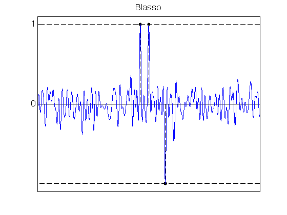
 
CBlasso - constructing the dual polynomial
% SDP CBLasso
lambda_max_CBlasso = norm(PhiS(fc,u,y),inf) /(norm(y)*sqrt(N))  ;
lambda_CBlasso = lambda_max_CBlasso/alpha ;
tic
cvx_precision best
cvx_solver sdpt3
cvx_begin sdp quiet
    variable X(N+1,N+1) hermitian;
    variable c(N) complex;
    X >= 0;
    X(N+1,N+1) == 1;
    X(1:N,N+1) == c .* conj(q);
    trace(X) == 2;
    norm(c)<= 1/(sqrt(N)*lambda_CBlasso) ;
    for j = 1:N-1,
        sum(diag(X,j)) == X(N+1-j,N+1);
    end
    maximize(real(c'*y))
cvx_end
toc

CBlasso_coeff = X(1:N,N+1);




% Plot the CBlasso polynomial

etaLambda_CBlasso = PhiS(fc,u,CBlasso_coeff);
figure(11) ;
hold on;
set(gca,'FontSize',16) ;
stem(x0, sign(a0), 'k.--', 'MarkerSize', ms, 'LineWidth', lw);
plot([0 1],  [1 1], 'k--', 'LineWidth', lw);
plot([0 1], -[1 1], 'k--', 'LineWidth', lw);
plot(u, etaLambda_CBlasso, 'b', 'LineWidth', lw);
axis([0 1 -1.1 1.1]);
set(gca, 'XTick', [], 'YTick', [0 1]); box on;
title('CBlasso')
Elapsed time is 25.498846 seconds.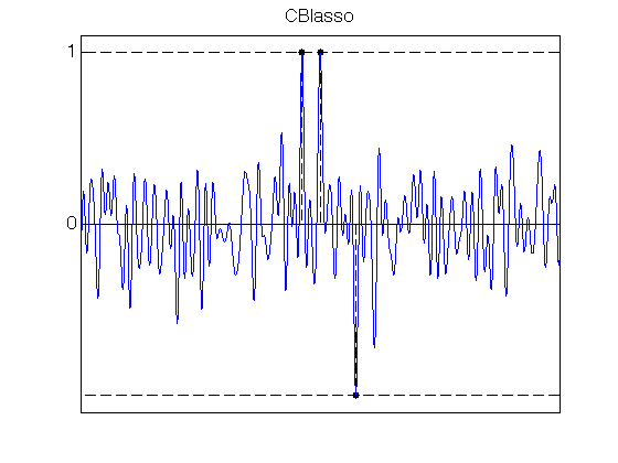
 
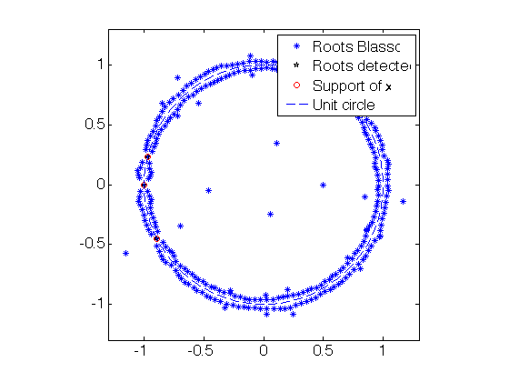
Roots-finding
tol = 1e-2 ;
% CBlasso poly
aux =- conv(CBlasso_coeff,flipud(conj(CBlasso_coeff))) ; % poly coeff of $- |p|^2$
aux(2*fc+1)=1+aux(2*fc+1);
roots_all_CBlasso = roots(flipud(aux)); % roots function convention


% CBlasso: Isolate roots on the unit circle
roots_CBlasso_detected = roots_all_CBlasso(abs(1-abs(roots_all_CBlasso)) < tol);
[~,I]=sort(angle(roots_CBlasso_detected));
roots_CBlasso_detected = roots_CBlasso_detected(I); % roots of 1-|p|^2
roots_CBlasso_detected = roots_CBlasso_detected(1:2:end); % roots of 1-|p


% Blasso poly
aux =- conv(Blasso_coeff,flipud(conj(Blasso_coeff))) ; % poly coeff of (- |p|^2)
aux(2*fc+1)=1+aux(2*fc+1);
roots_all_Blasso = roots(flipud(aux)); % roots function convention


% Blasso: Isolate roots on the unit circle
roots_Blasso_detected = roots_all_Blasso(abs(1-abs(roots_all_Blasso)) < tol);
[~,I]=sort(angle(roots_Blasso_detected));
roots_Blasso_detected = roots_Blasso_detected(I); % roots of 1-|p|^2
roots_Blasso_detected = roots_Blasso_detected(1:2:end); % roots of 1-|p



% Plot the complex roots
figure(20) ;
set(gca,'FontSize',16)
plot(real(roots_all_CBlasso),imag(roots_all_CBlasso),'*');
hold on;
plot(real(roots_CBlasso_detected),imag(roots_CBlasso_detected),'kp');
plot(cos(2*pi*x0), sin(2*pi*x0),'ro');
plot( exp(1i*linspace(0,2*pi,200)), '--' );
hold off;
legend('Roots CBlasso','Roots detected','Support of x','Unit circle'); axis equal; axis([-1 1 -1 1]*1.3);



figure(21) ;
set(gca,'FontSize',16)
plot(real(roots_all_Blasso),imag(roots_all_Blasso),'*');
hold on;
plot(real(roots_Blasso_detected),imag(roots_Blasso_detected),'kp');
plot(cos(2*pi*x0), sin(2*pi*x0),'ro');
plot( exp(1i*linspace(0,2*pi,200)), '--' );
hold off;
legend('Roots Blasso','Roots detected','Support of x','Unit circle'); axis equal; axis([-1 1 -1 1]*1.3);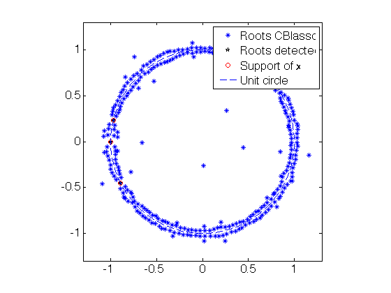
  
Solution via Blasso
% Precomputation for Blasso
x_Blasso = angle(roots_Blasso_detected)/(2*pi);
x_Blasso = sort(mod(x_Blasso,1));
Phix_Blasso = Fourier(fc,x_Blasso);
sign_coeff_Blasso = sign(real(Phix_Blasso'*Blasso_coeff));


% Lasso step
tic ;
lasso_sol_1 = (Phix_Blasso\y - lambda_blasso*pinv(Phix_Blasso'*Phix_Blasso)*sign_coeff_Blasso );
toc ;
Elapsed time is 0.002452 seconds.
Solution via Scaled lasso (alternating Lasso step and noise estimation)
% Precomputation for CBlasso
x_CBlasso = angle(roots_CBlasso_detected)/(2*pi);
x_CBlasso = sort(mod(x_CBlasso,1));
Phix_CBlasso = Fourier(fc,x_CBlasso);
sign_coeff_CBlasso = sign(real(Phix_CBlasso'*CBlasso_coeff));

% Alternating Lasso steps and noise estimations
tol = 1e-4 ;
maxiter = 1000 ;
niter = 0 ;
sigma_old = norm(y)/sqrt(N) ;
sigma_hat = 0.1 ; % initialization for $\hat{\sigma}$
tic ;
while (abs(sigma_hat(end) - sigma_old) > tol) && (niter<maxiter)
    niter = niter + 1 ;
    sigma_old = sigma_hat(end) ;
    lambda = sigma_hat(end) * lambda_CBlasso ;
    scaled_lasso_sol = (Phix_CBlasso\y - lambda*N*pinv(Phix_CBlasso'*Phix_CBlasso)*sign_coeff_CBlasso );
    sigma_hat = norm(y - Phix_CBlasso * scaled_lasso_sol)/sqrt(2*N) ; % should divide by sqrt(2)
end
toc ;
Elapsed time is 0.000915 seconds.
Comparison plot : reconstructed measures via Blasso and CBlasso
figure(100);
hold on;
set(gca,'FontSize',16)
stem(x0, a0, 'k.--', 'MarkerSize', ms, 'LineWidth', 1);
stem(x_Blasso, lasso_sol_1, 'ro--', 'MarkerSize', ms/2, 'LineWidth', 1);
stem(x_CBlasso, scaled_lasso_sol, 'b*--', 'MarkerSize', ms/2, 'LineWidth', 1);
axis([0 1 -1.1 1.1]);
legend('Original', 'BLasso','CBLasso');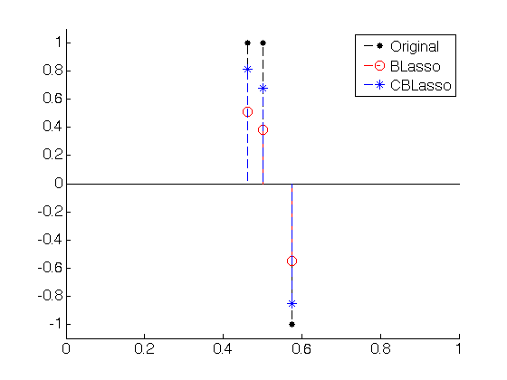
 
Noise estimation
sigma
sigma_CBlasso = norm(y - Phix_CBlasso * scaled_lasso_sol)/sqrt(2*N)  % divided by sqrt(2) due to the complex case
sigma_Blasso = norm(y - Phix_Blasso * lasso_sol_1)/sqrt(2*N)
sigma =

     1


sigma_CBlasso =

    0.9780


sigma_Blasso =

    1.1467


Published with MATLAB® R2014a